Instructions

TE Saturn is a non-commercial user-friendly software designed for the reduction and plotting of trace elements (TE) data. It is written in Python and runs independently, without the need for supporting commercial software.

In the TE Saturn Reduction, data files are individually processed, viewed, and interpreted in a combined set of interactive tables and graphical windows that display the (1) time-resolved signal and (2) all the corrected results. The display windows are interconnected and allow simultaneous visualization of plots and tables while the signal is being processed. This greatly improves the reliability of the data processing, particularly for very complex samples. A list of more than 1000 points can be processed online for different purposes (e.g. quality control) and offline.

In the TE Saturn Plot, TE data can be intelligently imported and plotted in ternary, line, and scatter graphs. A complete set of options permits several datasets to be plotted together and graphs to be customized to create publishable figures. All the graphs can be saved in various formats, including PNG, PDF, SVG, etc.

The software is free and available for download below. The source code for TE Saturn will be available on GitHub in the future, once procedures with patent registration are complete.

Videos on how to use the TE Saturn will be released soon. We are looking forward to seeing new users making good use of our LA-ICP-MS tool!

Downloading and Installing

TE Saturn does not need installation. It runs automatically from the folder below. It can be easily transferred from one computer to another without keys or an installation process. The TE Saturn’s executable file (i.e. .exe) comes with its database and icon files. We strongly advise users not to delete or move any file from this folder because this can cause the software to malfunction.

In the current version, TE Saturn only runs on Microsoft Windows platforms. A Mac platform version will be available in the future.

Download the TE Saturn here

In this version, it comes with a console window (back window) where the user can see eventual bugs. If some bug happens, we ask the user to take a print screen of this console and send it to us at geoquimicaisotopicaufop@gmail.com. Additionally, the .exe file may take a bit to open the first time you use it, so we ask the user to be patient.

Mean Features

The TE Saturn app was created for the reduction and plot of trace elements (TE) data. The two different functions are accessed in two separate interfaces chosen in the TE Saturn splash screen (Fig. 1).

Figure 1: TE Saturn splash screen where the user can access the Reduction and Plot interfaces

REDUCTION INTERFACE

The Reduction interface (Fig. 2a) is composed of a main control panel and four secondary windows. All five stages are interconnected allowing data visualization simultaneously in tables and graphs, resulting in a robust process of reduction.

The main control panel (Fig. 2a) is modern designed to provide an efficient and self-intuitive reduction environment. A broad range of operations is easily accessed in its left-side menu bar and all reduction status pop-ups in the bottom status bar. Calculations of element concentration are displayed in two separate tables, identified as Standard (RM) table and Sample (SP) table (Fig. 2b).

The RM table is designed to show all the corrected elements’ concentration, average and standard deviation on selected primary reference material analyses. The SP table displays corrected element concentration for samples and secondary reference materials. It also contains fields for Internal Standard (IS) values, which can be filled out individually for each selected spot analysis and automatically for all selected spots.

Selection of primary reference material spot analyses can be done in the list located on the left side of the RM table (Fig. 2b). While for samples and secondary reference materials spot analyses selections are done in the list neighbouring the SP table (Fig. 2b). Once the spots are selected, the software automatically runs calculations for elemental and downhole fractionation corrections and ppm concentrations, displaying the results.

Before selecting spot analyses for calculations, the user may select initial parameters, informing the software of the primary RM analysed and the IS was chosen for internal calibration. These parameters can be selected in the “Parameters and corrections” area (Fig. 2b), accessed by pushing the “Parameters” button in the left-side menu bar (Fig. 2a). Other optional parameters can be accessed in this area as well, such as drift correction, limit of detection (LOD) methodology and IS value format.

Figure 2a: TE Saturn’s main panel control, showing the left-side menu bar, status bottom bar and default central TE Saturn logo.

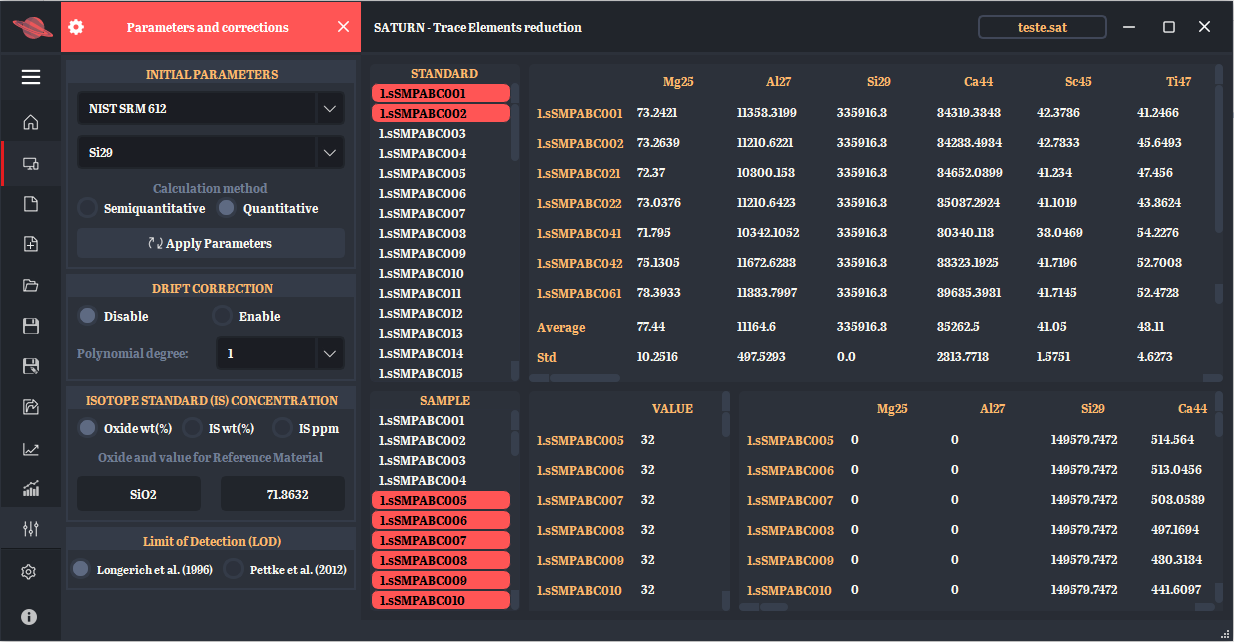
Figure 2b: TE Saturn’s main panel control, showing the Standard (RM) table (showing data for the NIST SRM 612), the Sample (SP) table (showing data for the Tanzania zircon; Santos et al., 2021), and the “Parameters and correlations” area.

The TE Saturn database already contains certified values of element concentration and matrix for the most commonly used RMs (e.g. NIST and USGS glasses). These values can be accessed in the Settings Window (Fig. 3), reached from the main left-side Menu (in Settings). The user can easily insert new certified values broadening the list of RMs in the database. They can also edit the certified values of any RM and even remove a RM from the database if it is needed.

Figure 3: The TE Saturn’s Settings window where the user can access the certified values for the most used reference materials (RM) and add data for new RMs or edit/remove previous ones.

TE Saturn also permits that the user to visualize and interact with the raw time-resolved data through the Time Series Window (Fig. 4), which plots the background and signal intensities for individual analyses against time. Besides visualizing the signal of individual analyses, the user has the option of plotting the time-resolved data of different analysed elements together in single cps-axis (elements in the same scale) and multiple cps-axes (elements in different scales) modes. More importantly, here the background and signal can be sliced in order to select the best areas of the time-resolved data. This graphic interface is linked to the RM and SP tables, therefore, the results are recalculated and displayed instantaneously after any small change in the signal and background slices.

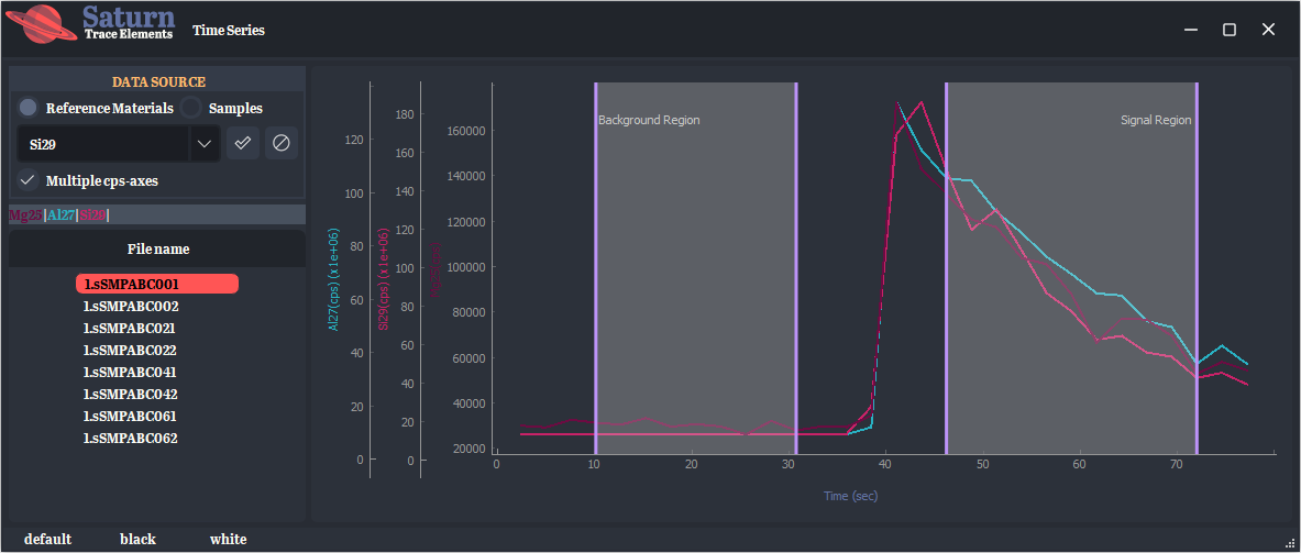
Figure 4: The TE Saturn’s Time Series window displaying the plot of the measured Mg25, Al27, and Si29 signal against time in the multiple cps-axis mode. The background and signal areas with which the user can interact and choose the better slices of the time-resolved data are also displayed.

The data reduced can be assessed in a second graphic window. The Plot Results Window (Fig. 5) displays options for binary, line, and ternary plots. A useful option for the calculation of the deviation from certified values is also available. The window reads and plots the analyses from the RM and SP tables. Key features such as normalization (e.g. chondrite, bulk earth, and mantle), log axes and whole plot configuration are easily accessed.

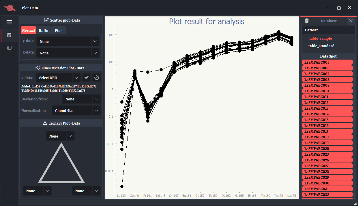
Figure 5: The TE Saturn’s Plot Results window showing a chondrite-normalized line plot of spot analyses of the Tanzania zircon (Santos et al., 2021). Besides line plot, the user can, here, plot data in scatter and ternary graphs, as well as assess the quality of the reduction of the primary and secondary reference materials through a deviation plot.

File Structure

TE Saturn reads LA-ICP-MS data files from ThermoFisher and Agilent mass spectrometers, including .txt, .FIN2, and .csv file extensions. As ICP-MS output data files vary in extension and format, the software identifies and uses specific import data modules that convert them into TE Saturn generic format. A primary requirement is that individual spot analyses should be exported in separate output files –a feature that is easily set in most mass spectrometers. Once loaded, the software instantaneously reads the file and recognizes the masses. For each of the measured masses, it creates a databank with stored information from the background and signal.

If your ICP-MS data output is not supported, please contact us at geoquimicaisotopicaufop@gmail.com and send us some of your data files and we will build up a module for your equipment data format.

Data Processing

The raw data from individual analyses are processed in time-resolved mode and, here, any fraction of the entire period of one analysis is called a time-slice. The software automatically separates the time-resolved signal into two time-slices: (1) background and (2) signal (Fig. 4). The background signal region relates to the baseline detection at a particular mass, and the sample signal is the additional counts from the ablated sample material. Thus, the main data input requirement is that each raw data file should include background and signal information for all measured masses.

TE Saturn has a feature that recognizes the rise of the time-resolved (IS mass) signal of individual analyses and automatically separates the background signal and sample signal. The range of each signal area can be easily modified by the user via the graphic interface that plots the signal against time (Time Series Window; Fig. 4)

The individual masses are then averaged and transformed into background-subtracted signals. The calculations are done internally for all imported files. Finally, the background-subtracted signals are converted into ppm concentrations following the methodology of Longerich et al. (1996) according to the user selection in the RM and SP lists in the main control panel. The Limit of Detection (LOD) for each mass and analysis is also calculated. In that case, the user can choose between the Longerich et al. (1996) and Pettke et al. (2012) methodologies selecting either option at the “Parameters and corrections” area (Main Window; Fig. 2b).

PLOT INTERFACE

The Plot interface (Fig. 6) is characterized by a robust main panel and a secondary window (Fig. 7) that handles data importation. In the Plot interface, the user can construct binary, lines, and ternary plots. Options for plotting classification diagrams of various minerals are in development and will be completely operational in the future.

TE Saturn Plot has an intelligent module created to automatically identify features and read the imported data. This is especially useful when plotting multi-sample data.

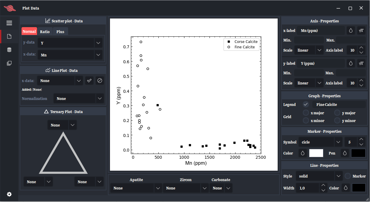
Figure 6: The TE Saturn Plot’s main panel control shows in the centre a scatter plot of calcite trace elements, a left-side menu bar, plot options and graph properties on the left and right side of the central area, respectively.

The Import Data window is accessed by pushing the “Import Data” button located in the main left-side menu bar (Fig. 6). The selection of the data file to import is done using the top options of the window (Fig. 7) and a preview of the imported data is displayed in the central table. The only requirement is that the file to be imported must be an Excel file saved with the .csv extension.

In the preview table, the user has the option to edit the data structure dropping unnecessary rows or columns. In addition, the data file may contain several data separated into different worksheets; these can be selected in the “worksheet” box (Fig. 7).

Figure 7: The TE Saturn Plot’s Import Data window shows imported data in the preview table and a list of the worksheets contained in the imported file.  

After hitting the import button, the user must first inform in which direction the data header is located, choosing the “Elements direction” option in the popped-up window (Fig. 8). Then, the software runs its intelligent module over the data file characterizing all the data structures. Finally, the user can split the data into different datasets, if it is needed, name the dataset(s), and import it.

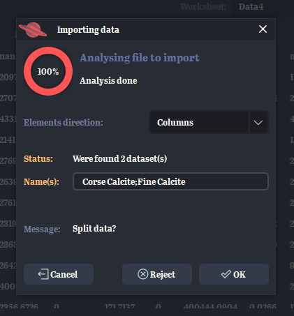
Figure 8: A TE Saturn Plot’s dialogue window that pops up when the import button is pushed. In this pop-up dialog, the user first informs the software of the data header direction and the intelligent module shows all information found about the file structure. Knowing this information, the software can split the data into datasets and save it in the database.

The imported datasets are saved and listed in the Database area of the main panel (Fig. 6), reached from the Database button of the Menu. Datasets can be plotted separately or together according to the user’s wishes. Additionally, the user can choose to plot a dataset entirely or just slice it. All these options are done by selecting the data accordantly to the Database area.

All the plot options are located on the left-side of the central plot area (Fig. 6). Scatter plot graphs can be created by axing two elements, the sum of elements or/and the ratio of elements. Normalized line graphs can be done, in this case, to chondrite, bulk earth, and mantle. Plot with three axes is also available through the Ternary Plot options.

A complete configuration of the graph features can be found on the right-side of the central plot area (Fig. 6). The user can customize the axes by changing the scales, the ranges, and the size of the tick labels; can customize the axes labels choosing the letter style, colour, and size. All the graph area is also customized such as the legend and the grids. Additionally, how the data is shown in the plot can be personalized by choosing the markers and line properties for each dataset plotted.

All the plots in the TE Saturn Plot can be saved through a right-mouse-button click (Fig. 9). An export option allows the user to save the plots in PNG, JPEG, PDF, SVG, and TIFF formats.

Figure 9: Examples of different graphs plotted, customized, and imported from the TE Saturn Plot interface.